Graphs
When performing experimental work, we test the hypothesis and measure observable quantities. Often, we also plot graphs to demonstrate a relationship between the results and our theory.
A graph plots the relationship of one quantity against another on two axes at right-angles to each other. Usually, we have control over one of the quantities and this is known as the independent variable, the other quantity is determined by the outcome of the experiment or some mathematical relationship. We call this the dependent variable because it depends on the independent variable. We usually plot the independent variable on the x-axis and the dependent variable on the y-axis.
Common Graphical Relationships
The Straight Line Graph
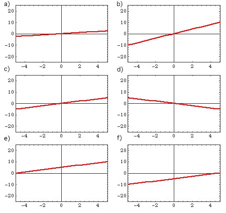
The equation for a straight line is y = mx +c (1)
Where y is the dependent variable, m is the gradient or slope of the graph, x is the independent variable and c is the intercept this is the value at which the line crosses the y-axis.
The gradient is determined by the (change in y)/(change in x) or m = (y2-y1)/(x2-x1) = Δy/Δx.

Quadratic Relationship
If the independent variable, x has a relationship that depends on the x2 then it is a quadrative dependence.
y = ax2 + bx + c(2)

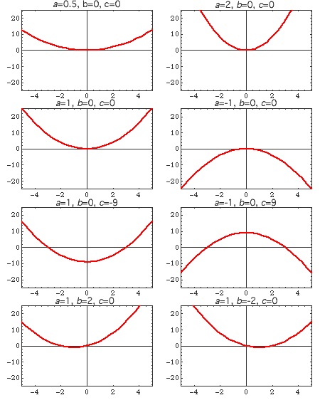
The quadratic dependence has three separate variable and so can produce a variety of parabolas. Figure 2. show some of the behaviours for different values of a, b, and c. The a variable controls how quickly the parabola increases with x. If it is positive the parabola goes up and is trough-shaped as in example a). A negative value of a inverts the parabola as in b). the variable c controls the height of the parabola on the y-axis. c) shows the a positive value of a and a negative value of c which makes the parabola dip below the x-axis y-region between x=±3. d) shows a negative value for a and a positive value for c which make the parabola rise into the positive y region between x=±3
In examples, g) and h) we set c = 0 and a = 1. The value of b controls the sideways displacement of the parabola. If b is 0, then the parabola is symmetric about the y-axis. A negative value of b shifts the parabola to the left while a positive value shifts the parabola to the right. The degree of shifting is half the value of b. Thus for a value of ±2 the shift is 1 unit to the right or left, respectively.
Exponential Graph

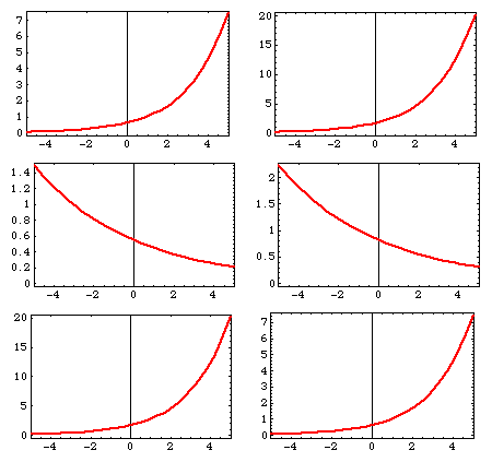
Curves following exponential growth or decay occur in many areas of physics such as the charging and discharging of capacitors, or in the decay of radioactive material.
A general exponential growth is represented by
y =k exp(ax)(3)
A general exponential decay is written,
y = k exp(-ax)(4)
Where y is the dependent variable, k is a multiplying constant, a is a positive constant and x is the independent variable.
Straight Line Graphs
A straight-line graph is the most useful type of graph to show the relationship between the dependent and independent variable. It allows one to see a glance, how well the experimental data-points fit the predicted behaviour. It is possible to convert the different types of curve we have discussed to have a linear relationship.
For a quadratic relationship, it is possible to plot a straight-line as long as the curve is symmetric about the y-axis. i.e. b = 0 in equation, (2). In this case, we plot y against x2, c will the intercept, (the point on the y-axis when x = 0). a will be the gradient of the curve.
Since the natural log is the inverse function of an exponential function, ln(exp(x)) = x. Therefore, an exponential curve can be changed into a linear relationship by taking natural logs of both sides of (3). A refresher of logarithms is given here.
ln(y) = ax + ln(k) (5)
Similarly, taking logs of (4) gives,
ln(y) = ln(k) - ax (6)
This has the same form as a straight-line with gradient a and intercept ln(k) if we plot ln(y) against x.
The same procedure works when the dependent variable has the form of a power law. For example, if we have a graph has the following form: y = axk. It can be turned into the same form as a straight-line graph by taking logs to the base 10 of both sides.
This gives, log10(y) = log10(a) + k log10(x).
This is now also in the form of a straight-line graph by plotting log10(y) against log10(x). The gradient is k with log10(a) for the intercept.
